QIPGraph manual

QIPGraph is a set of C++ libraries and Excel interfaces to interact with gnuplot, a fast command line driven graphic software. Using QIPGraph, you can create complex graphics with a few simple lines of C++ or in Excel.

Gnuplot has many advantage, in particular it accepts file commands which allows you to save and scale your work. This article is a typical example where I was able to use almost the same script with different datas to make the 64 figures.

1.2 Version

Current version 1.0, March 2012

1.3 Installation

How to install QIPGraph on your computer.

Download gnuplot. Current last version: gp444win32.zip or check at gnuplot download
Extract the files in the folder C:\Program Files\gnuplot. It is important to have this folder since the Excel Add-in will look into it to get the executable.
Download QIPGraph.zip and extract all files in the folder C:\Program Files\QIPGraph.
Open Excel and install the add-in using Tool – Add-Ins – Browse to load the file C:\Program Files\QIPGraph\ QIPGraphGUI.xla.
C++ interface: The header files, .lib, and .dll are in the directory C:\Program Files\QIPGraph. There are no dependencies to any other library apart STL.

1.4 C++ Interface

This interface allows gnuplot to be controlled from C++. It is designed to be minimal. In this way the knowledge of gnuplot is almost sufficient to learn how to use the library.

1.4.1 Example

We begin by an example.

#include "C:\Program Files\QIPGraph\QIPGraph.h"

#include <vector>

using namespace QIPGRAPH;

int main()

{

// create instance

bool persist = false; // gnuplot does not persists after end of program

int width = 300; // width of the plot window

int heigh = 200; // width of the plot window

Plot plot(persist,width,heigh); // get an instance of gnuplot

// plot function

plot.command("p cos(x)" ); // fig 1

// create data, 3 columns

std::vector<double> vec_x, vec_y, vec_z;

vec_x.push_back(-1.); vec_x.push_back(2.); vec_x.push_back(3.);

vec_y.push_back(1.3); vec_y.push_back(2.); vec_y.push_back(1.);

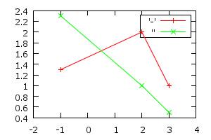
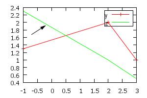
vec_z.push_back(2.3); vec_z.push_back(1.); vec_z.push_back(0.5);

// send data directly to gnuplot

// plot 2 curves in the same figure

plot.command("p [-2:4] '-' w lp, '' w lp" );

plot.plot_Vectors("",vec_x, vec_y);

plot.plot_Vectors("",vec_x, vec_z); // fig 2

// change dir, need special command to update current dir in Plot class

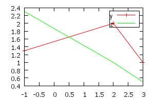
plot.command_cd(" cd 'C:\\Documents and Settings\\dami\\My Documents'");

// save to a file first

plot.plot_Vectors("data3.dat",vec_x, vec_y, vec_z);

// plot from file

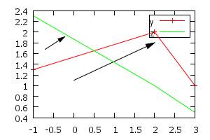
plot.command("p 'data3.dat' u 1:2 w lp t 'y','' u 1:3 w l t 'z'" ); // fig 3

// plot arrow using the mouse

// click on the initial position, push “5” to store the position

// click on the final position, push “5” to store the position

int number = 1; // number of the arrow

plot.command_arrow(number); // fig 4

// plot arrow giving positions (from, to) = (0,1.1) to (2,1.8)

std::string style = "";

number = 2;

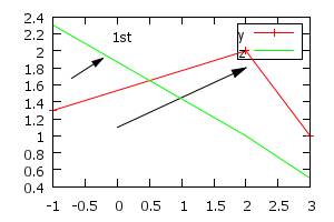
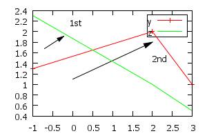
plot.command_arrow(number,style.c_str(),0,1.1,2,1.8); // fig 5

// plot label using the mouse

// click on the position, push “5” to store the position

number = 1;

style = "";

plot.command_label("1st" ,number, style.c_str()); // fig 6

// plot label giving coordinates: (2,1.8)

number = 2;

style = "";

plot.command_label("2nd" ,2,style.c_str(),2,1.5); // fig 7

// obtain MOUSE_X variable (last click)

double MOUSE_X = plot.get_value_double("MOUSE_X");

// obtain a vector of values

std::vector<const char*> vecMouseVar;

vecMouseVar.push_back("MOUSE_X");

vecMouseVar.push_back("MOUSE_Y");

vecMouseVar.push_back("MOUSE_X2");

vecMouseVar.push_back("MOUSE_Y2");

vecMouseVar.push_back("TOTO"); // not present

std::vector<double> vecMouse = plot.get_value_double(vecMouseVar);

// result = { MOUSE_X, MOUSE_Y, MOUSE_X2, MOUSE_Y2, NaN_d)

return 0;

}

Remark: the shortcut “5” on plot windows is defined as the beginning of the session.

Fig 1:

1.4.2 Interface

The interface has no dependency to any other program. It consists only of the header file QIPGraph.h . Basically it contains a function to send command and another to send the vectors either to gnuplot or to a file.

1.4.2.1 Namespace

All the variables and functions are declared in the namespace QIPGRAPH

namespace QIPGRAPH

1.4.2.2 Create instance

Plot(const bool& keep_ = false, const int& width_ = 300, const int& height_ = 200)

bool persist // gnuplot does not persists after end of program

int width // width of the plot window

int heigh // width of the plot window

Example

Plot plot()

1.4.2.3 Send a command

Plot& command(const char* command_);

Plot& command_cd(const char* command_);

The command_cd is here to update some internal directory for the Plot class needed when saving a file.

Example:

plot.command("p 'data3.dat' u 1:2 w lp t 'y','' u 1:3 w l t 'z'" );

1.4.2.4 Sending vectors

Send vectors either to gnuplot (if filename =0 or empty) or to a file.

Plot& plot_Vectors(const char* filename_,

const std::vector<double>& vec1_

, const std::vector<double>& vec2_ = std::vector<double>()

, const std::vector<double>& vec3_ = std::vector<double>()

, const std::vector<double>& vec4_ = std::vector<double>()

, const std::vector<double>& vec5_ = std::vector<double>()

, const std::vector<double>& vec6_ = std::vector<double>()

);

Example:

// save to a file first

plot.plot_Vectors("data3.dat",vec_x, vec_y, vec_z);

// send data directly to gnuplot

plot.plot_Vectors("",vec_x, vec_y);

1.4.2.5 Label and Arrow

These functions are convenient but not absolutely necessary since you can directly the command function:

Plot& command_arrow(const int& n_=-1, const char* style_="",const double& xFrom=NaN_d, const double& yFrom=NaN_d, const double& xTo=NaN_d, const double& yTo=NaN_d);

Plot& command_label(const char* label_, const int& n_=-1, const char* style_="",const double& xFrom=NaN_d, const double& yFrom=NaN_d );

Mainly used to plot arrow and label using the mouse. Recording the last click using “5” shortkey and then send the command. Example:

plot.command_arrow()

plot.command_label("label")

1.4.2.6 Query to gnuplot

We have several functions to get variables from gnuplot. However if it is quite easy with an Unix OS, it is very difficult to get a bidirectional interface with gnuplot under Windows OS. Our solution is therefore quite slow when quering values from gnuplot and should be avoided on Windows, if possible.

// bidirectional, avoid using for Windows

std::string get_value_string(const char* variable_, const char* type_ = "s");

std::vector<std::string> get_value_string(const std::vector<const char*>& variables_, const char* type_ = "s");

double get_value_double(const char* variable_);

std::vector<double> get_value_double(const std::vector<const char*>& variables_);

If the variable is not defined a Nan_s or Nan_d constant is returned. The user must check the return value against these values before using it.

1.4.2.7 Set paths

We can change the current folder into gnuplot using the command:

Plot& command_cd(const char* command_);

This is equivalent as to send two commands

Plot& command_cd(const char* command_);// send commang in gnuplot

void set_current_dir(); // set gnuplot folder in the class

We can also query the current dir:

std::string get_current_dir() // get dir stored in the DLL

We can set and query the path of gnuplot.exe:

QIPGRAPH_API void set_path_exe(const std::string& path_exe_);

QIPGRAPH_API std::string get_path_exe();

These functions are global in the namespace QIPGRAPH

We can set and query the path of the temporary folder where some temporary files are written:

QIPGRAPH_API void set_path_temp(const std::string& path_exe_);

QIPGRAPH_API std::string get_path_temp();

These functions are global in the namespace QIPGRAPH

1.5 Excel Interface

Gnuplot can be a good supplement to Excel plotting.

You have installed QIPGraph GUI add-in as explained in the installation procedure.

The best way is to use the QIPGraph GUI form.

1.5.1 Excel Functions

Even though the QIPGraph form is the best way to interact with gnuplot, you can still send commands directly from Excel.

There are several functions available

1.5.1.1.1 PlotCreate

PlotCreate(string Name, bool keep, int width, int height, bool force)

Keep = persist = keep gnuplot open after closing excel

width and height of the window plot

force = force to create a new gnuplot

see Create instance:

1.5.1.1.2 PlotPermanent

String_handle PlotPermanent(string xlHandle_, string xlName_)

Used in VBA to create a permanent object, otherwise the next creation of a Plot object will overwrite it by default. This feature is necessary to avoid memory leaks.

1.5.1.1.3 PlotRemove

Void PlotRemove(string xlHandle_)

Used in VBA to remove Plot object when they are permanent.

1.5.1.1.4 PlotCurrentDir

String_handle PlotCurrentDir(string xlHandle_)

Get current directory of the DLL and gnuplot.

1.5.1.1.5 PlotCommand

String_handle PlotCommand(string xlHandle_, string xlCommand_)

Main function. See Send a command:

1.5.1.1.6 PlotCommand_arrow

String_handle PlotCommand_arrow(string xlHandle_, int xlN_, string xlStyle_)

Used to plot arrow from mouse clicks.

See Label and Arrow.

1.5.1.1.7 PlotCommand_label

String_handle PlotCommand_label(string xlHandle_, int xlN_, string xlLabel_, string xlStyle_)

Used to plot label from mouse clicks.

See Label and Arrow.

1.5.1.1.8 PlotVec

String_handle PlotVec(string xlHandle_, string xlfilename_, Range xlVec1_, Range xlVec2_, Range xlVec3_, Range xlVec4_, Range xlVec5_, Range xlVec6_)

Plot vector to gnuplot or save to file, see Sending vectors.

1.5.2 QIPGraph GUI Add-in

1.5.2.1 Excel menu

You have access to a right click mouse menu:

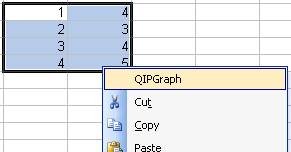
This will launch the QIPGraph GUI.

1.5.2.1 QIPGraph Form

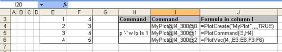
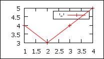
If more than 2 cells are selected, as shown in the figure, QIPGraph will try to plot the two columns as (x,y).

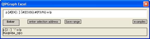
The QIPGraph form is shown below

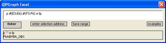
It is composed of a “command line” similar to the one in gnuplot. This command line is associated to a parser to replace the #( ):#( ) by the values of the ranges in the active spreadsheet. Therefore the command

p #(E3:E6):#(F3:F6) w lp

corresponds in C++ to:

command(p ‘-‘ lp) // shown in the lower box

plot_Vec(,Range(E3:E6),Range(F3:F6))

If you type a command you can get the range format #( ):#( ):#( ) by

select the range in the spreadsheet
use the button below “enter selection address”

If you are interesting in a value of the cell instead of a range, use the string #[ ]. Example

p [ #[E4] : ] #(E3:E6):#(F3:F6) w lp

means

command(p [2:] ‘-‘ lp) // shown in the lower box

plot_Vec(,Range(E3:E6),Range(F3 :F6))

1.5.2.2 Save file

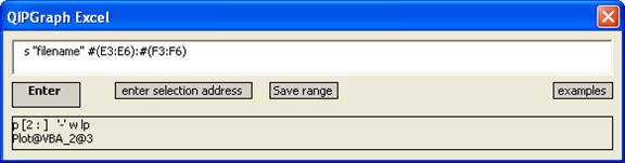
You can type the command or select the range and push the button “save range” to write the command. You have to update the “filename”, and send the command.

1.5.2.3 Editing

When pushing the key “Enter”, the string will be sent to the parser, and then the corresponding commands will be sent to gnuplot through the QIPGraph DLL, and the plot generated by gnuplot.
You can use a historic of the commands using the Up and Down keys.

1.5.2.4 Examples Button

The Button “Examples” opens a web page with your default browser with some examples of gnuplot command.

Moreover, in the QIPGraph GUI you can use the command cd … directly. The parser will take care of sending the two commands to the dll.

1.5.2.5 VBA programming

You can use all functions defined in the Excel interface. When creating a Plot object in VBA, you have to call PlotPermanent function to avoid to be overwritten by the next creation of object. When you do not need it anymore, use PlotRemove to release the memory. Example:

Dim GraphId As String

GraphId = Application.Run("PlotCreate") // create temporary plot

GraphId = Application.Run("PlotPermanent", GraphId) // avoid overwrite

Application.Run("PlotRemove", GraphId) // remove when not need anymore

1.6 FAQ

1. I do not know gnuplot programming, could I use this interface?

Yes. Gnuplot is very easy to learn. You can see several examples below.

2. I need to start twice gnuplot from C++ or Excel to let it works, Is it normal?

This is due to a problem in the speed of initializing gnuplot. We are working on this problem.

3. When querying a gnuplot variable, why do I get an error even if it exist?.

Querying it again should solve the problem. The bidirectional interaction is difficult on Windows OS. This will be improved in the next version.

3. ExcelAdd-in does not seems to work?

Reduce the security of your excel to “medium”

1.7 TODO

- Unix implementation

- Print function.

- Better communication from gnuplot to C++.

- Possibility to read a vector with errors.

- Excel: Possibility to select n>2 columns to plot

- Delay problem to load gnuplot the first time from DLL

1.8 Gnuplot commands

“Clean examples”. I tried to be as simple as possible to understand the main features.

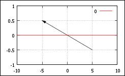
1.8.1 Arrows

# number from-to head type style

set arrow 1 from 5,-0.5 to -5,0.5 head filled size screen 0.03,15 linewidth 1 linetype rgb "black"

# set arrow 1 to 1,1 # change head

p 0

http://www.gnuplot.info/demo/arrowstyle.html

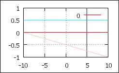
1.8.2 Lines

# from-to type color

set arrow 2 from graph 0, first 0.5 to graph 1, first 0.5 nohead linewidth 1 linetype rgb "cyan" # horizontal

set arrow 3 from 5,-1 to 5,1 nohead linewidth 1 linetype rgb "blue" # vertical

set arrow 4 from graph 0,0.5 to graph 1,0 nohead # from graph coordinates

p 0

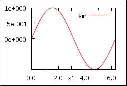
1.8.3 Axes

set xtic 2 # every 2

set ytics 0,0.5 # from 0, every 0.5

set ytics nomirror # do not show tics at the right

set xtics add("x1" 3) # add one tic “x1” at 3

set format x "%.2f" # 2 decimals for x

set format y "%1.0e" # exp format for y

set mxtics 2 # minor x tics frequency = 2

p [0:2*pi] sin(x) t "sin"

# set xtics ("NE" 72.0, "S" 42.0, "Downtown" 12.0, "Suburbs" 122.0) # define xtics on axe x

# set format x "" # no number for x axis

set zeroaxis # plot axis , xzeroaxis, yzeroaxis

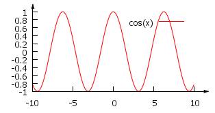
1.8.4 Axes with arrows

set border 3 # border left + bottom

set tics nomirror # no tics on right and top

set arrow 1 from graph 1,0 to graph 1.09,0 size screen 0.02,15,60 filled # axe x + type arrow

set arrow 2 from graph 0,1 to graph 0,1.09 size screen 0.02,15,60 filled # axe y + type arrow

set tmargin at screen 0.90 # otherwise margin calculated automatically

set rmargin at screen 0.90 # and not sure to see arrows

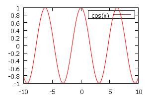
p cos(x)

1.8.5 Axe time

set xdata time # set axis time format

set format x "%d/%m/%y %H:%M:%S" # display

set xtics 5*24*60*60 rotate by -60 in # frequency in seconds: 5 days, rotate -60 degres, inside tics

set xrange ["01/06/2003":"21/06/2003"] # time does not see to work

p cos(x) # time = seconds from 01 january 2000

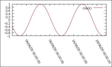
http://www.gnuplot.info/demo/timedat.html

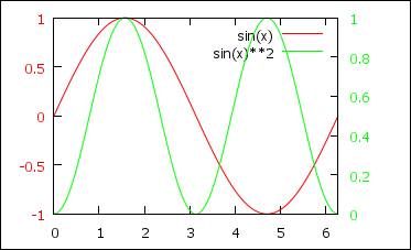
1.8.6 Two y axes

set ytics nomirror # not same tics left and right

set ytics -1, 0.5 textcolor rgb "red" # left tics from -1 with 0.5 interval

set y2tics 0, 0.2 textcolor rgb "green" # right tics from 0 with 0.2 interval

set y2range[0:1] # right axis range

p [0:2*pi] sin(x) lt rgb "red" axis x1y1,sin(x)**2 lt rgb "green" axis x1y2 # plot and choose color of figures

http://www.gnuplot.info/demo/multiaxis.html

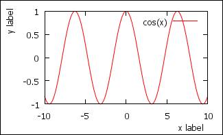
1.8.7 Axes label

set xlabel "x label" offset graph 0.4,0.05 # standard: center, move to the right

set ylabel "y label" rotate by 90 offset graph 0,0.4 # standard center, move to the top

set ytics 0.5 # 0.5 interval

p cos(x)

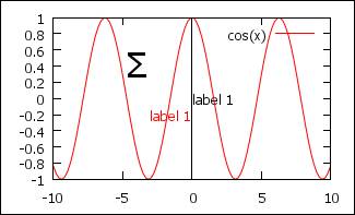
1.8.8 Label

set label 1 "label 1" at 0,0 left # label from

set label 2 "label 1" at 0,-0.2 right textcolor rgb "red" # label to

set arrow 2 from first 0, graph 0 to first 0, graph 1 nohead # to see the diff

set label "S" at graph 0.3,0.8 center font "Symbol,24" # sigma "Time-Roman,12"

http://www.gnuplot.info/demo/enhanced_utf8.html

http://www.gnuplot.info/demo/textrotate.html

http://www.gnuplot.info/demo/textcolor.html

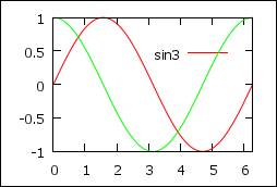
1.8.9 Legend

set key off # no legend

set key 4,0.6 left # legend from (4,0.6)

p [0:2*pi] sin(x) t sprintf("sin%d",3),cos(x) notitle # using C format, no title for second function

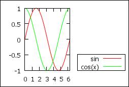
You can choose to put the legend outside:

set key below # below the figure

set key above # above the figure

set key outside right # outside right bottom

set key box lt rgb "black" lw 1 # box around legend

# set key spacing 0.7 # reduce spacing between legend, but pb with box

p [0:2*pi] sin(x) t “sin”,cos(x)

set key invert # invert order of legend = same if invert order of plot

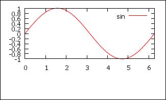
1.8.10Margin

set bmargin 5 # bottom, can be “l”, “r” or “t”, useful to align multiplots

p [0:2*pi] sin(x) t "sin"

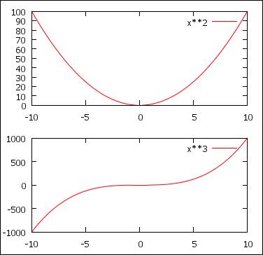
1.8.11Multiplot 1

set multiplot layout 2,1 # two rows, 1 col

set lmargin 6 # to aligne the two figures

p x**2

set lmargin 6 # to aligne the two figures

p x**3

unset multiplot # stop multiplot mode, otherwise plot new curves on the top

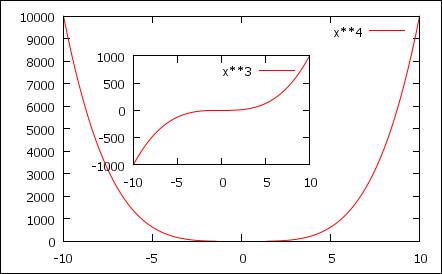
1.8.12Multiplot 2: insert

set multiplot # enter multiplot mode

p x**4

set rmargin at screen 0.70 # right margin at 0.7 in the screen

set lmargin at screen 0.30 # left margin at 0.3

set bmargin at screen 0.40 # bottom margin at 0.4

set tmargin at screen 0.80 # top margin at 0.8

p x**2 # plot insert

http://www.gnuplot.info/demo/multiplt.html

http://www.gnuplot.info/demo/layout.html

http://www.gnuplot.info/demo/margins.html

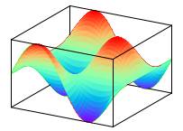
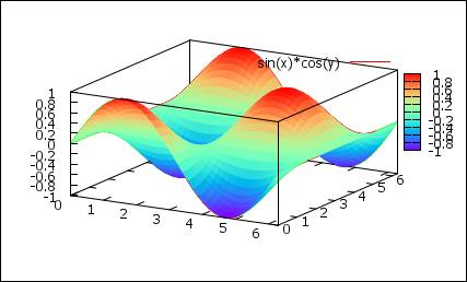
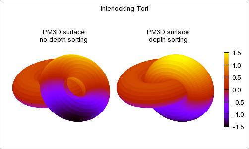
1.8.133D plot

set ticslevel 0. # z start at 0, (default=0.5)

set isosample 40,40 # more accurate surface (default 10)

set hidden3d # do not show hidden surface

set pm3d at s # s = normal, b = surface

set palette rgbformulae 33,13,10 # change color

set border 4095 # to see all borders until the top

# set grid z # if you need grid for z

sp [0:2*pi] [0:2*pi] sin(x)*cos(y)

set pm3d map # map 3d to 2d

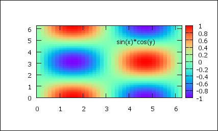
set pm3d s # go back to normal surface

set view # 2d to 3d

sp [0:2*pi] [0:2*pi] sin(x)*cos(y) # get the first figure in 3d

http://www.gnuplot.info/demo/

1.8.14Candelstick

http://www.gnuplot.info/demo/candlesticks.html

1.8.15Steps

http://www.gnuplot.info/demo/steps.html

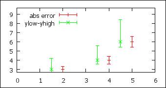
1.8.16Error bars

set key left # legend at the left of the graph

set xrange [0:6]

p 'data1.dat' u 1:2:($2/10) w e t "abs error"\

,'data1.dat' u ($1-0.5):2:($2*9/10):($2*14/10) w e t "ylow-yhigh" # x:y:y_low:y_up

data1.dat

1.8.17Bar chart / histogram 1

set boxwidth 0.9 relative # size relative to the default

set style data histograms # bar

set style fill solid 1.0 border -1 # with border , see help border for options

p 'data1.dat' u 2,'' u 3 # show 2 bars for each row

data1.dat

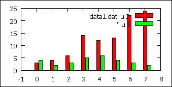
http://www.gnuplot.info/demo/histograms.html

1.8.18Bar chart / histogram 2

p 'data1.dat' u 1:2:($2*0+0.8) w boxes notitle # last column = size of the boxes = 0.8

data1.dat

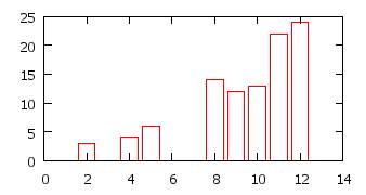
http://www.gnuplot.info/demo/histograms.html

1.8.19Fit

f(x) = a*x + b # function to fit

fit [1:6] f(x) 'data1.dat' via a,b # fit in the range [1,6] only

p 'data1.dat',f(x)

data1.dat

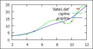
1.8.20Smooth

p 'data1.dat'\

,'' u 1:2:(1.0) w lp smooth csplines t "cspline"\

,'' u 1:2:(1.0) w lp smooth acsplines t "acspline" # (1.0) = weight

data1.dat

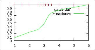
1.8.21Cumulative

# Useful to plot the cumulative of a serie of random results from probability distribution

# data2.dat

# 1 1

# 3 1

# 2 1

# 3.1 1

# …

p 'data2.dat' ,'' u 1:(1/13):(1.0) w lp smooth cumulative t "cumulative" # 13 datas, (1.0) = weight

data2.dat

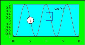
1.8.22Rectangles, circles, and background

# background with rectangle

set object 1 rectangle from screen 0,0 to screen 1,1 behind fc rgb "green" # full screen rectangle, behind all other

set object 2 rectangle from graph 0,0 to graph 1, 1 back fc rgb "cyan" fillstyle solid 1.0 # graph background

set object 3 rect from 0,0 to 2,0.5 fs empty border rgb "blue" # small rectangle, empty, border blue

set object 4 circle at -3*pi/2,0. size 1 fs transparent border rgb "black"

p cos(x)

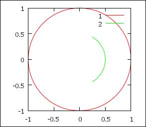
1.8.23Parametric

set size ratio 1 # size screen x = size screen y

set parametric # enter parametric : variable t

set trange [-pi:pi] # set range for parametric

set xrange [-1:1] # range for x

set yrange [-1:1] # range for x

fx(t,r,c) = r*cos(t/c) # function -> x, r = radius, c = to vary parametric range

fy(t,r,c) = r*sin(t/c) # function -> y, r = radius, c = to vary parametric range

plot fx(t,1,1),fy(t,1,1) t "1",fx(t,0.5,3),fy(t,0.5,3) t "2" # 2^nd from –pi/3 to pi/3, radius = 0.5

http://www.gnuplot.info/demo/param.html

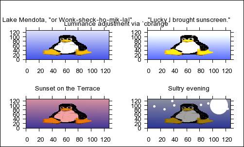
1.8.24Styles

1.8.25Plot and command window

p cos(x) # plot cos(x)

plot 'file.dat' e 10 # plot only 1/10 of the points: e=every

p 'data1.dat' u 1:2,'' u 1:3 # '' = same file

set sample 10 # x interval by 10 for function f(x), decrease for more accurate

set label "test" at first 0,0.5 # can be first, second, graph, screen, or character

clear # clear figure

reset # reset to default the set

replot # redo last command plot, reread data

refresh # redo last command with memory, do nor=t read again data

pause 2 # pause 2 s

1.8.26Plot window

# Shortcuts:

# space = from plot window to command line

# g : toggle grid

# wheel : translate y

# shift+wheel : translate x

# ctrl+wheel : zoom

# ctrl+shift+wheel: zoom x

bind c 'print "great"' # shortcut: print “great” when hitting c in plot windows

pause mouse "Click" # pause until click on window plot

lower 0 # lower window 0

raise 0 # raise window 0 to the top of the windows

test # show possibilities of the terminal

# Mouse

print MOUSE_X

print MOUSE_Y

print MOUSE_X2

print MOUSE_Y2

print MOUSE_BUTTON

print MOUSE_KEY

print MOUSE_SHIFT

print MOUSE_CTRL

print MOUSE_ALT

pause mouse keypress # pause until key is pressed
print "Keystroke ", MOUSE_KEY, " at ", MOUSE_X, " ", MOUSE_Y

# min max values for the graph

print GPVAL_X_MIN

print GPVAL_X_MAX

print GPVAL_Y_MIN

print GPVAL_Y_MAX

1.8.27Terminals

# eps -> latex

set term postscript eps enhance

set terminal postscript eps enhanced color font 'Helvetica,10'

# set terminal epslatex size 8.89cm,6.65cm color colortext

# http://www.gnuplotting.org/introduction/output-terminals/

# http://www.gnuplot.info/docs/tutorial.pdf

set output "test.eps"

# pdf

set term pdf

set output "test.pdf"

# png

set term pngcairo

set terminal pngcairo size 350,262 enhanced font 'Verdana,10'

set output "fig.png"

#wxt : default windows

set term wxt

set term wxt 0 size 300,200 # window number 0, size (height*width=) 300*200

set output

# to save and restore previous term

set term push # remembers the current terminal including its settings

set term pop # restores it

1.8.28Strings manipulations

print "A"."B" # "AB"

graph(n) = sprintf("Title for plot #%d",n) # function with C format

p cos(x) title graph(4) # plot with “title for plot #4”

http://www.gnuplot.info/demo/stringvar.html

http://www.gnuplot.info/docs_4.2/gnuplot.html#x1-7000019

1.8.29Scripts and Macros

#Write the last two mouse click positions using a bind to key

bind 5 load 'mouse_keep_1.gnu' # when pressing ‘5’ in plot window, load macro in the file

and the macro file “mouse_keep_1.gnu” is below. Each time the program is loaded, it will

1. push the last position of the mouse (mouse_x_b,mouse_y_b) to (mouse_x_a,mouse_y_a)

2. push the last click position into (mouse_x_b,mouse_y_b)

3. print the result on the screen

4. same for second axes if they exist.

if(defined(MOUSE_X)) if(defined(mouse_x_b)) mouse_x_a=mouse_x_b;else mouse_x_a=0;

if(defined(MOUSE_X)) mouse_x_b = MOUSE_X;

if(defined(MOUSE_X)) if(defined(mouse_y_b)) mouse_y_a=mouse_y_b;else mouse_y_a=0;

if(defined(MOUSE_X)) mouse_y_b = MOUSE_Y

if(defined(MOUSE_X)) print "(",mouse_x_a,mouse_y_a,")"

if(defined(MOUSE_X)) print "(",mouse_x_b,mouse_y_b,")"

if(defined(MOUSE_X)) print "(",mouse_x_a,mouse_y_a,")"

if(defined(MOUSE_X)) print "(",mouse_x_b,mouse_y_b,")"

if(defined(MOUSE_X)==0) print "MOUSE_X not defined, please click on the graph";

if(defined(MOUSE_X2)) if(defined(mouse_x2_b)) mouse_x2_a=mouse_x2_b;else mouse_x2_a=0;

if(defined(MOUSE_X2)) mouse_x2_b = MOUSE_X2;

if(defined(MOUSE_X2)) if(defined(mouse_y2_b)) mouse_y2_a=mouse_y2_b;else mouse_y2_a=0;

if(defined(MOUSE_X2)) mouse_y2_b = MOUSE_Y2

if(defined(MOUSE_X2)) print "(",mouse_x2_a,mouse_y2_a,")"

if(defined(MOUSE_X2)) print "(",mouse_x2_b,mouse_y2_b,")"

With this you can load another macro to plot an arrow between the last two mouse positions:

set arrow from mouse_x_a,mouse_y_a to mouse_y_b,mouse_y_b

you could use a more direct way using the mouse event with some if/else conditions:

pause mouse "Click" # pause until click on window plot

1.8.30Save / load

save 'work.gnu' # save current session

load 'work.gnu' # load session

1.8.31Write to file

command=sprintf("echo %f > toto.txt",MOUSE_X) # define “echo ‘MOUSE_X’ > toto.txt”

system command # execute command, here write MOUSE_X in “toto.txt”

print GPVAL_PWD # current directory

http://news.gmane.org/gmane.comp.graphics.gnuplot.user

1.9.4 Links

http://www.gnuplot.info/demo/

http://t16web.lanl.gov/Kawano/gnuplot/index-e.html

http://www.gnuplotting.org/

http://gnuplot-tricks.blogspot.com/

1.9.5 Google

gnuplot on google